Citations:
Atanas Kamburov, Konstantin Pentchev, Hanna Galicka, Christoph Wierling, Hans Lehrach, Ralf Herwig (2011)
ConsensusPathDB: toward a more complete picture of cell biology.
Nucleic Acids Research 39(Database issue):D712-717.
Atanas Kamburov, Christoph Wierling, Hans Lehrach, Ralf Herwig (2009)
ConsensusPathDB--a database for integrating human functional interaction networks.
Nucleic Acids Research 37(Database issue):D623-D628.
For questions and comments regarding ConsensusPathDB, please contact Dr. Atanas Kamburov: kamburov@molgen.mpg.de.
Introduction
ConsensusPathDB is a database that integrates different types of functional interactions between physical entities in the cell like genes, RNA, proteins, protein complexes and metabolites in order to assemble a more complete and a less biased picture of cellular biology. Currently, ConsensusPathDB
contains metabolic and signaling reactions, physical protein interactions, genetic interactions, gene
regulatory interactions and drug-target interactions in human, mouse and yeast. The interaction information is collected from 30 public
resources and is integrated into a seamless network.
Physical entities from the source databases
are mapped to each other on the basis of common
identifiers like UniProt and Entrez accession numbers.
Interactions with matching primary participants
(i.e., substrates and products in the case of biochemical
reactions, interactors in the case of protein interactions and
regulated gene in the case of gene regulatory interactions) are
also mapped and grouped together according to similarity.
The database content is updated every three months
with the newest available versions of the source databases; new source databases are integrated at the rate of 1-2 databases per release.
The functionalities of the ConsensusPathDB web interface are described below.
Database content information
Clicking on the link "content information" on the left panel of the ConsensusPathDB start page will take you to a summary of the current interaction content in the database. Most notably, the entity and interaction overlap tables summarize the number of unique physical entities and interactions present in each integrated resource, as well as the number of overlapping interactions and physical entities between resources. Figure 1 below shows the overlap tables for Release 1 of ConsensusPathDB as an example.
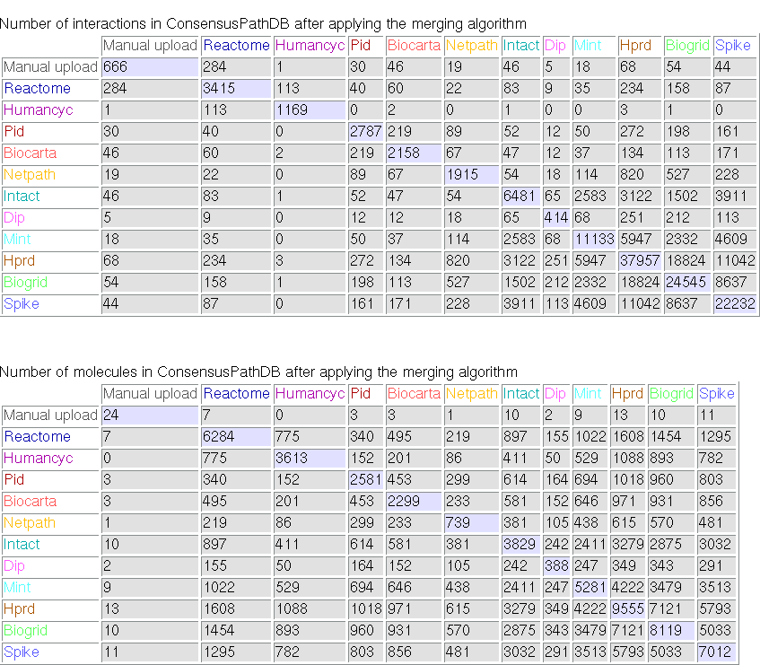
Figure 1
Overlap tables showing the number of overlapping interactions and physical entities across functional interactions resources (ConsensusPathDB release 1, 12.12.2007). The numbers in the diagonal denote the numbers of unique interactions and physical entities present in source databases, respectively. Example: the HumanCyc database contains 1169 unique interactions involving overall 3613 unique physical entities. Of these, 113 interactions and 775 physical entities are also present in the Reactome database.
Search in ConsensusPathDB
One way to access the integrated interaction information in ConsensusPathDB is to search for specific interactions. Currently, the web interface to ConsensusPathDB offers two possibilities to do this.
Search interactions of specific molecules or pathways
The ConsensusPathDB user can search for interactions of specific physical entities or pathways.
First, search terms are provided in the form of trivial names or accession numbers (e.g., UniProt or KEGG
accession numbers). It is possible to search for multiple physical entities or pathways simultaneously by
entering query keywords in separate rows. Search results summarize the names of matching objects and,
if the objects have been searched by accession numbers, the accession numbers matching the query.
Additionally, external web links are provided for each hit that show the origin of the physical entity
or pathway, and navigate the user to the web site containing the original information about the according item. Normally, pathways have only one external link (because pathways from
different resources are not compared with each other), and physical entities may have multiple links (because
matching physical entities from different resources are merged in
ConsensusPathDB).
After selecting relevant pathways or physical entities, their
functional interactions are listed. If the selected
pathways contain subpathways or if the physical entities
constitute groups, e.g. protein families, then the interactions
of the subpathways or group members, respectively, are also listed.
At this stage, each
interaction that is displayed has a single source. The user is
able to specify mapping criteria according to which similar
interactions are to be merged. Interactions
with matching primary participants are considered
similar. Which interactions should be considered identical,
depends on the user's settings: the user is able to
specify whether the primary participants of similar interactions must have
matching modification patterns, subcellular localization and/or
matching stoichiometry (in the case of biochemical reactions) in
order the similar interactions to be considered identical. According to these settings,
interactions are merged together and displayed in the visualization environment
of ConsensusPathDB which is described below.
Apart from the standard search for interactions of physical entities or pathways, the web interface of ConsensusPathDB features searching for the shortest path(s) of functional interactions that link a couple of physical entities with each other. Here, the user specifies a path "start" and a path "end". One possible shortest path between both is calculated and displayed (Figure 2.). The user is able to exclude particular physical entities from the shortest path, which is especially useful when non-specific hubs like ubiquitin and ATP are present in the path. Interaction paths of interest can be visualized in the visualization environment of ConsensusPathDB, which is described below.
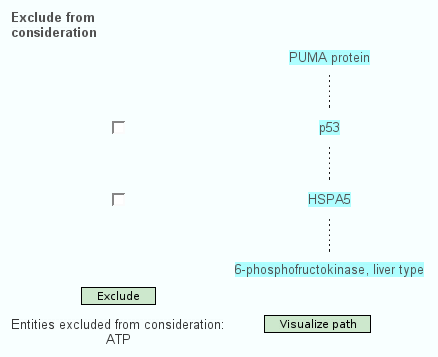
Figure 2
One shortest path of functional interactions linking PUMA with PFKL, excluding ATP. The path involves 4 proteins: PUMA, P53, HSPA5 and PFKL. A dashed line between one physical entity and the next indicates that there is at least one functional interaction containing the two proteins. If P53 and/or HSPA5 are excluded, another shortest path will be calculated that does not involve these proteins. A detailed interaction network-graph showing the type and the origin of relevant interactions linking the physical entities is shown by clicking on "Visualize path".
Interaction network visualization environment
Interaction networks can be viewed in an interactive visualization environment. The web interface user has two choices for a visualization environment: an image-based visualization and a visualization based on Cytoscape.js. Both frameworks display interaction networks in the same style so switching between them involves barely any user acclimatization. The image-based visualization is no longer supported and will be removed soon. The newer, Cytoscape.js visualization environment allows much more flexibility, e.g. it allows the user to pan, zoom, and re-arrange the networks. Notably, gene / protein expression data can be overlaid on the nodes of a currently viewed network to enable the interaction network based interpretation of such data. Here, we describe the common features of both visualization environments.
Elements of ConsensusPathDB interaction networks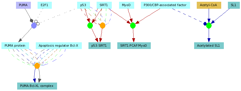
Figure 3
An example functional interaction network automatically generated by the visualization environment of ConsensusPathDB. The network contains three biochemical reactions (green circles), two protein-protein interactions (orange circles) and one gene regulatory interaction (purple circle) involving overall seven proteins (light blue rectangles), five protein complexes (darker blue rectangles), a metabolite (light brown rectangle) and a gene (purple rectangle). Multiple edges connecting the functional interaction nodes (circles) with the physical entity nodes (rectangles) show that the interactions have multiple sources coded by the edge colors. The role of each interaction participant is denoted by the edge style and arrow shape (see Figure 4. for details)
Functional interaction graphs displayed in ConsensusPathDB (example in Figure 3.)
contain two types of nodes (bipartite network) and several types of
edges. Both nodes and edges differ in their shape and
color. Rectangular nodes represent physical entities (genes,
proteins, compounds, etc.) and circular nodes represent interactions
between nodes. The color
of physical entity nodes shows the type of the physical
entity, and the same is true for interaction nodes. For example,
biochemical reactions are shown as green circles, and physical
interactions are shown as orange circles. The primary name of each
physical entity in the graph is displayed inside the representing
node by default. Post-translational modifications and subcellular locations
of physical entities are shown in square brackets behind the name, if
the user has chosen those as differentiation criteria for interaction
mapping when visualizing selected interactions of entities or pathways. Edges linking an
interaction participant with the according interaction node also differ
in their style, arrow shape, and color. The edge style and arrow
shape indicate the role of the according physical entity in the
interaction. The origin of interactions is indicated by the edge
color: multiple edges with the same style and arrow shape but
with different colors may exist between a physical entity and an
interaction, indicating that the interaction is present in multiple
databases. Encoding origin information as an edge attribute
(i.e. edge color) and not as an interaction attribute
allows more detailed attribution of origin information: think for
example of an interaction which is present in two different databases
but for which different enzymes are provided in each database.
A detailed graph legend is available in the visualization environment and is shown by
clicking on the graph legend link from the menu panel of the
visualization environment (Figure 4.).
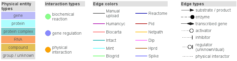
Figure 4
Legend of the interaction network-graphs generated by the visualization environment of ConsensusPathDB.
Visualization facilities
The visualization environments of ConsensusPathDB provide several functionalities to give entity and interaction information details and facilitate graph viewing. Synonymic names of interactions and physical entities are shown in tooltips when pointed at with the mouse cursor. For physical entities, external database identifiers are also displayed in the tooltip. Protein complex compositions are displayed instead of trivial complex names by clicking on the node representing the complex and selecting "switch to component view". For the static-image based visualization framework, we have implemented a JavaScript tool that mimics the hand-tool of other well-known viewing software like e.g. Ghostscript viewers and Adobe Reader. To scroll the graph using the hand-tool, just click anywhere on a white space in the graph and move the mouse while holding down the left mouse button. Another facility which ensures convenient work with larger graphs is the locate tool: you can locate any molecule present in the graph by entering a name or an accession number in the input field at the top right corner of the visualization environment page.
Interactive modification of interaction networks
Interaction network-graphs displayed in the visualization
environment are dynamical. Not only can the visibility of certain
interactions' participants be toggled, but interactions can be
added or removed from the graph.
The names of physical entities that are normally shown inside the
rectangles representing the according physical entities can be
hidden, which is especially useful when the user wishes to hide
the names of certain, less important entities in the interaction
graph thus stressing on the rest of the present objects. Moreover,
physical entities with a secondary role (e.g. enzymes, modifiers)
can be hidden, for example when the user wishes to visualize only
the mass flow in a biochemical pathway. The visibility of
names and of complete physical entity nodes can be toggled for
single physical entities by clicking on the according node with
the left mouse button and selecting the appropriate option from
the tooltip menu, or for all physical entities in the
network-graph by choosing the appropriate options from the
visibility settings menu at the menu panel in the top
region of the visualization environment page.
Apart from manipulating existing physical entity nodes, the user
can hide single interactions, lists of interactions or connected
components of the graph (again by choosing according options on
the tooltip menus of nodes or the options from the menu
panel). New interactions can be added to the interaction graph by
expanding physical entity nodes with their further interactions
(left-click on an entity node -> expand node in the tooltip
menu) or by searching for physical entities or pathways that are
possibly not present in the graph, and selecting their
interactions of interest (menu panel -> misc functions ->
add interactions).
The user can always undo his last graph modification by
clicking on undo last graph changes button on the menu
panel.
For interaction networks displayed in the visualization
interface, the user can view a summary of the number of physical
entity and interaction nodes of specific types, as well as an interaction
mapping summary. To access this feature, click on misc
functions in the menu panel -> network statistics.
Visualization graphs can be exported from the visualization
environment by clicking on misc functions (in the menu
panel) -> export network. Several possibilities are
provided: the interaction network-graph can be exported as a
graphics file in several formats, including png, jpg,
postscript and others, as a BioPAX file or as a ConsensusPathDB model
dump. BioPAX is an XML-based file format that carries information
on interaction systems and is currently supported by many
software packages for e.g. biochemical system modeling. The
ConsensusPathDB model dump can be imported into the visualization
environment (see Section File upload and mapping) and worked
with at a later time point. Model
dumps can be imported only if the ConsensusPathDB version has not
changed in the meantime.
Molecular concept-based analysis of gene/metabolite lists
ConsensusPathDB offers two statistical approaches to analyze user-specified lists of genes or metabolites obtained e.g. by microarray experiments or mass spectrometry, respectively. The first approach is over-representation analysis, where predefined lists of functionally associated genes (pathways, Gene Ontology (GO) categories and neighborhood-based entity sets, explained below) are tested for over-representation in the user-specified list based on the hypergeometric test. The second approach is based on the Wilcoxon signed-rank test and takes as input genes with exactly two measurement values, typically expression values in two distinct phenotypes. While the over-representation functionality typically takes as input a relatively short, non-weighted list of "special" (e.g., differentially expressed) genes, for the Wilcoxon enrichment analysis approach, genome-wide expression data containing measurements of possibly thousands of genes are the preferred input.
The molecular concept-based analysis aproaches are detailed below (although they are explained on the basis of input lists of genes, the same applies for metabolite lists).
The user can provide a list of identifiers of interesting genes or proteins, e.g. of genes that are significantly over-
or underexpressed in a certain phenotype compared to a control phenotype. The gene identifiers are mapped to physical entities in ConsensusPathDB.
Over-represented sets are searched among currently three categories of predefined gene sets: network neighborhood-based sets,
pathway-based sets and Gene Ontology-based sets. For each of the predefined sets, a p-value is calculated according to the hypergeometric test based on
the number of physical entities present in both the predefined set and user-specified list of physical entities. If no
background is uploaded by the user (corresponding to the list of IDs of all measured entities in the experiment), the
background parameter value for the hypergeometric test will depend on the type of the accession numbers used for the
input list: more precisely, the background size is the number of ConsensusPathDB entities that are anotated with an ID of
the type the user has provided, and participate in at least one pathway / GO category / neighborhood-based entity set (depending on
which of these predefined classes are considered by the user). The size of the tested predefined sets is also
corrected to the number of set members that are annotated with an ID of the user-specified ID type (since the rest of the
set members can never occur in the candidates list, using the specific namespace). This "effective" set size is provided in the analysis results in brackets after the absolute size. The p-values are corrected for
multiple testing using the false discovery rate method and are available as q-values on the results page. Sets whose hypergeometric p-value
passes the threshold defined by the user are listed, and for each set, the set size (the absolute size, as well as the corrected size), the over-representation p-value, the q-value, the set size and all
interaction resources contributing to the construction of the set are provided. The set definition in terms of set
centers in the case of neighborhood-based sets (see below), pathway name in the case of pathway-based sets or GO category name in the case of GO category over-representation are also
displayed. For sets with a reasonable size, more details like the list of all set members and the list of interactions
connecting the physical entities can be viewed. In the case of neighborhood-based sets and pathways, bar charts are displayed that summarize the GO cellular
component, molecular function and biological process annotations (flattened to GO level 2) of the members of the according set. Each of the three charts shows the five most common annotations from the according GO category. For each entity set
of reasonable size, the underlying interaction network-graph can be viewed in the ConsensusPathDB visualization
interface, where physical entities from the uploaded list are marked with a red border.
Neighborhood-based sets are sets of physical entities that are connected to each other with one or more functional interactions. Each neighborhood-based set has a central physical entity (or simply a center) and a radius denoting the maximal distance in terms of number of interactions separating the center from the rest of the entities in the set. The distance between physical entities involved in some functional interaction is 1. The same is true also for enzymes catalyzing neighboring biochemical reactions (i.e. reactions that have common primary participants, e.g. when a product of the first reaction is a substrate in the second). To avoid redundancy in sets, we allow sets to have more than one center, and merge sets with different centers that have the same members.
We have predefined a large number of neighborhood-based sets, according to different centers and radii. The user can choose to search for enriched neighborhood-based sets with a radius of 1 or 2 interactions and can additionally impose constraints on the nests like minimal size (i.e. minimal number of different proteins and genes contained in the set), minimal connectivity index, minimal overlap with the input list, and p-value. The connectivity index, which quantifies the level of interconnectedness within neighborhood-based sets, is defined as the fraction of all real interaction edges of all possible edges connecting the entities in the set, which is k*(k-1)/2 for a set of size k.
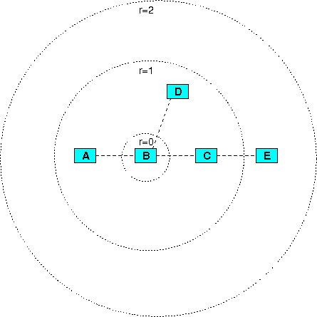
Figure 6
An example for neighborhood-based sets. Assume that four interactions exist, the first between molecules A and B, the second between B and C, the third between B and D, and the fourth between C and E. These define several neighborhood-based sets according to the set center and the radius: for example, the set with center B and radius 1 contains A, B, C and D (i.e. the set center B and its next neighbors A, C and D), the set with the same center but with radius 2 contains A, B, C, D and E (the set center B, its next neighbors A, C and D, and B's second-next neighbor E).
Apart from neighborhood-based entity sets, ConsensusPathDB contains pre-defined pathway-based sets from several pathway databases. A pathway-based set contains all the proteins and genes that are involved in a curated biochemical pathway. Gene Ontology (GO) based sets contain genes that are together annotated with a specific GO term. In ConsensusPathDB, GO categories from levels 2 and 3 of the GO hierarchy are available for pathway analysis. Complex-based sets are sets of genes whose protein products are members of the same annotated protein complex.
Wilcoxon enrichment analysisThe Wilcoxon enrichment analysis method carries out a paired Wilcoxon signed-rank test for each NEST / GO category / pathway based on the user-specified measurement values of its members. The measurement values for every gene / protein, uploaded by the user, typically reflect genome-wide gene expression or proteome-wide protein abundance in two different phenotypes. For every uploaded gene or protein, exactly two values must be supplied in the input form (or uploaded file). The Wilcoxon test assignes a P-value to each functional set based on how probable it is that the combined measurement differences of genes in the functional set between the phenotypes have appeared by chance. Q-values are calculated using the same method as in the over-representation analysis approach.
Visualization of molecular conceptsThe typical output of most tools for gene/metabolite set over-representation/enrichment analysis is a table where the different molecular concepts (e.g. pathways) are listed, ranked according to some statistical measure of association with the user-specified gene/metabolite list (most often a P-value). However, the molecular concepts often overlap with each other to some extent - for example, they may stand in a hierarchical relationship to each other (like Reactome pathways and Gene Ontology categories) or may share key elements. In the latest version of ConsensusPathDB, we have thus introduced the possibility to visualize the different molecular concepts (pathways, neighborhood-based sets, Gene Ontology categories and protein complexes), resulting from a particular over-representation or enrichment analysis, as concept overlap graphs (Figure 7). In these graphs, each node represents a separate concept whose member list size (i.e., number of genes/metabolites contained) and P-value are encoded as node size and node color, respectively. Two nodes are connected by an edge if they share members. The edge width reflects the relative overlap (corresponding to the Fowlkes-Mallows index) between the nodes, while the edge color encodes the number of shared members that are also found in the user's input (denoted "shared candidates"). This visual representation helps the user to quickly identify related biological processes that together show a changed activity, e.g. because they have the same key regulators. Moreover, it gives a quick overview over the relationships between the different types of concepts (e.g., particular Gene Ontology biological process categories may be very similar to particular pathways contained in pathway databases). Last but not least, the color coding of edges can provide clues about potentially dysregulated crosstalks between different biological processes. The overlap graph visualization environment features a filter that can be applied to edges in order to highlight only the closest relationships between concepts.
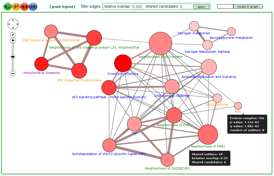
Figure 7
Molecular concepts shown as an overlap graph.
Induced network modules analysis
In addition to the over-representation/enrichment analysis of predefined molecular concepts, the web interface of ConsensusPathDB provides another approach for the interaction- and pathway-centric analysis of lists of genes, called induced network modules analysis. The approach was first proposed in Berger et al., 2007. Given a list of so-called seed genes (e.g. resulting from microarray experiments, which are unable to directly disclose the functional relationships between genes), it aims to interconnect those genes through different types of interactions (physical, biochemical, regulatory, etc.; selectable by the user). This information on the pairwise functional/physical relationships between the genes can shed light e.g. on the biological reasons why they are identified together in the experiment. For example, if a group of genes found to be over-expressed in a microarray experiment are highly interconnected through physical interactions, this suggests that those genes may encode proteins which together form a protein complex that has a high concentration in the phenotype under study and thus may be relevant for this phenotype.
Notably, the induced network modules may optionally include genes that are not in the user-supplied seeds list, but associate two or more seed genes with each other and overall have significantly many connections within the induced network module (purple nodes in Figure 8 below). These so-called intermediate genes are likely to be associated with the phenotype under study, although they may not be regulated on the transcriptional level and thus do not appear in the input gene list. For example, if a group of seed genes are all connected through gene regulatory interactions to an intermediate node that represents a transcription factor, this suggests that the transcription factor may be dysfunctional (e.g. due to a mutation, which does not necessarily impact the transcription factor's expression). Intermediate genes are ranked according to the significance of association with the seeds list given their overall connectivity in the background network. This is quantified by a z-score calculated for each intermediate node with the binomial proportions test. The z-score threshold can be controlled dynamically by the user in order to create sub-networks involving many intermediate and seed genes with a less stringent threshold or more compact sub-networks with a more stringent threshold.
If numerical values (e.g. expression values) are available for the genes, they can be uploaded and overlaid on the nodes of the resulting induced modules to allow an easier interpretation.
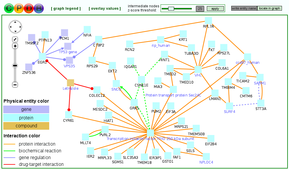
Figure 8
An example unduced module. Nodes with black labels are seed genes/proteins, nodes with purple labels are intermediate nodes.
Network upload
Through the web interface of ConsensusPathDB, users can upload interaction networks in BioPAX, PSI-MI or SBML format. Upon upload, physical entities and functional interactions are compared against the content of ConsensusPathDB. .This is done based on identifiers (UniProt, KEGG, ChEBI, ...) in the case of physical entities and on participant composition in the case of interactions. The uploaded networks are visualized, and for interactions present in ConsensusPathDB, the source databases are displayed. Networks can be expanded in the context of the database content by adding further interactions, and edited.
SBML files should have physical entity annotations as in the BioModels model repository
More information
Licensing information
The use of CPDB is free of charge for academic users. Commercial users should contact Dr. Ralf Herwig ( herwig [at] molgen.mpg.de ). Data stored in ConsensusPathDB is available under the license terms of each contributing database.
DisclaimerAlthough best efforts are always applied, the developers of ConsensusPathDB do not assume any legal responsibility for correctness or usefulness of the information in ConsensusPathDB.
AcknowledgementsConsensusPathDB is being developed by the Bioinformatics group of the Vertebrate Genomics Department at the Max-Planck-Institute for Molecular Genetics in Berlin, Germany. The project was supported by the EMBRACE and CARCINOGENOMICS projects that are funded by the European Commission within its 6th Framework Programme under the thematic area "Life Sciences, Genomics and Biotechnology for Health" (LSHG-CT- 2004-512092 and LSHB-CT-2006-037712); 7th Framework Programme project APO-SYS (HEALTH-F4-2007-200767); German German Federal Ministry of Education and Research within the 65 NGFN-2 program (SMP-Protein, FKZ01GR0472); Max Planck Society within its International Research School program (IMPRS-CBSC).
For more information, please contact kamburov[at]molgen.mpg.de .